
The power of Bayesian thinking & big numbers.
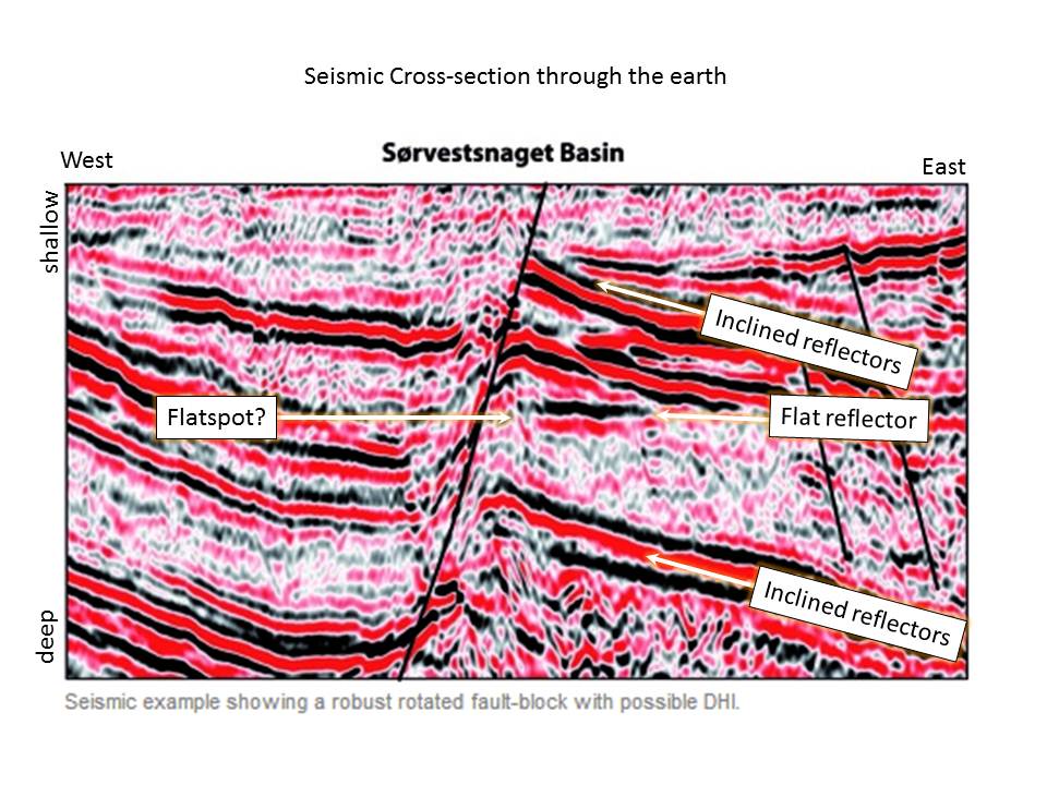
So, you’re an exploration manager at an oil company. You have identified 50 structures on seismic data and applied some detailed geophysical analysis to confirm that some of them have a Direct Hydrocarbon Indicator, or DHI. In this case it is what is known as a “flat spot”, or a seismic reflector that corresponds to a fluid contact in the subsurface.
Have you found a multi-million barrel oilfield?
Surprisingly, the answer is not immediately intuitive. No oil exploration evidence is conclusive: there are always false negatives and false positives. To have a chance of answering the question correctly you need to know three pieces of information:
- the background likelihood that a structure in the region could contain oil
- the chance that a flatspot would correctly identify the structure as an oilfield if oil was present
- the chance that a flatspot would incorrectly identify the structure as an oilfield if oil was not present.
In this case, you think that around 1 in 5 structures in the region contain oil (20%). Furthermore, you know that a flatspot correctly identifies an oilfield 60% of the time, and incorrectly identifies a dry structure as an oilfield 30% of the time.
So, when you observe a flat-spot, have you found an oilfield?
If you have not come across this sort of question before, take a moment to think about it.
What’s your answer?
….
….
In fact it is unlikely that you are now JR, rolling in dollar bills. In this example you would actually have a 1 in 3 chance of having correctly identified an oilfield, or 33.3%.
The reasoning is quite simple. Out of the 50 potential oilfields, 10 are expected to contain oil (20%). The flatspot will correctly identify 6 of these (60% of those with oil). However, the flatspot also has a 30% false positive rate, which means that 30% of the remaining 40 structures (12), look like they have oil in them.
So, in total 18 structures look like they have oil in them due to having a flatspot. But only 6 of these actually have oil in them. That’s just 1 in 3, or 33%. Furthermore, 4 of the structures without flatspots will also be oilfields, or 8% of the total.
The observation of a flatspot does not mean you have an oilfield, but it does mean that your chance of finding one using this technique shifted from 1 in 5 if drilling blind, to 1 in 3 using seismic analysis.
This is Bayesian statistics in action.
A more commonly cited Bayesian example is the “do you have cancer” calculation. This is fantastically explained by Eliezer S. Yudkowsky on his blog at the Machine Intelligence Research Institute (http://yudkowsky.net/rational/bayes)
To summarise Yudkowskuy, if you’ve tested positive for cancer, do you have cancer?
In the Yudkowskuy case all you know is that the incidence in the population of this type of cancer is 1%, and that 80% of those with cancer will be detected by the test. In addition, it is known that the test also provides a false positive in 9.6% of cases.
Well, whilst most doctors presented with this test answered incorrectly, it is in fact extremely unlikely that you are ill in this example. You would actually have less than a 1 in 10 chance of having the disease, or 7.8% to be exact.
Again, the reasoning is quite simple. Out of the 10,000 people tested, 100 are expected to have cancer (1%). The test will correctly identify 80 of these (80% of those with cancer). However, the test also has a 9.6% false positive rate, which means that 9.6% of the remaining 9,900 people who don’t have cancer, or a whopping 950 people, are also told they are positive.
So, in total 1,030 people test positive for cancer, but only 80 of the positive tests actually have the disease. That’s just 7.8%. Furthermore, 20 of the 8,970 that tested negative will be surprised to find they are actually ill (a far smaller 0.2%).
Bayesian statistics
The proportion of structures identified that are likely to contain oil, or the proportion of people tested for cancer who are likely to have the disease are the prior probabilities. The aim of additional evidence in the form of a geophysical flat-spot observation or a medical test is to help polarise the original population into two groups: those with a higher likelihood of the outcome than the prior probability, and those with a lower likelihood than the prior probability.
As we’ve noted, observations and tests aren’t full proof. Their outcomes don’t completely replace the initial prior probability, but simply modify it. In the presented cases the evidence was provided by a low reliability geophysical observation or a moderately reliable medical test. The chance that a structure with oil in it or a patient with cancer is correctly identified by the observation or test, and the chance that a structure without oil in it or a patient who doesn’t have cancer is given a false positive are known as the conditional probabilities. The critical piece of information that is often forgotten when thinking intuitively about these problems is the likelihood of a false positive. Ignoring false positives that exist in any noisy dataset will lead to a wildly inaccurate estimate of true probability.
Collectively the prior probability and the two conditional probabilities are known as priors. You need all three pieces of information to assess the true likelihood of a given outcome using Bayesian techniques.
The final answer is called the revised probability, or posterior probability.
As you may have noticed, the prior probability is a strong controller of the outcome. Nature doesn’t know what your prior probabilities are, and doesn’t care, so getting a good handle on them so that they are as close to reality as possible is really useful. The two examples illustrate different levels of uncertainty in the prior probability. In the oil industry it is very difficult to say with confidence that a structure in a given area has a certain probability of working. In contrast, medical studies have a much better handle on the statistical likelihood of being ill in any given population.
We are not made for statistical thinking
So let’s think on another statistical conundrum.
This time you are on a game show. The presenter, Monty Hall, explains the new game. He shows you three doors. Behind one door is a car, and behind the other two doors is a goat.
He asks you to pick a door. You pick the 1st door.
At this point Monty Hall tells you how great the prize car is, and opens up another door, the 3rd, to show you that it has a goat behind it. He then asks you if you’d like to stick with your first guess, the 1st door, or switch to door number 2.
Is it to your advantage to switch your guess to the 2nd door?
…
Intuitively it seems to make no difference whether you switch your choice of door or not. But what happens when you think about this probabilistically?
The answer is that switching doubles your chances of winning from 1 in 3, to 2 in 3.
Weird, huh!
Why?
The initial probability of picking the correct door is 1 in 3. That is, you have a 1 in 3 chance of picking the car before any other information is given. However, once you are shown a goat behind door number 3, there are just a couple of outcomes left. Either you correctly picked the car first time, which was a 1 in 3 chance, in which case switching guarantees that you will lose, or you initially picked a goat, which was a 2 in 3 chance, and then by switching you will select the door with the car, as you are unable to select the goat that has already been shown to you.
It is perhaps best to show this graphically.

Counter-intuitive eh?
http://en.wikipedia.org/wiki/Monty_Hall_problem

